Summary: This article discusses the effects of public debt on private investment activity. The research is based on an econometric approach, which analyses theoretical determinants of private investment including level of public debt, as a potential determinant. Potential effects of public debt on private investment is essentially important in modern world, as most governments tend to overhang debt and sometimes it can be obstacle for the private sector.

Key words: Public Debt, Private Investment, Debt Overhang. 

Introduction

Most governments in the modern world use borrowed resources to finance their operation related to the infrastructure development or merely current needs. Despite positive sides of financing government operations with borrowed sources, sometimes there can be a tradeoff between governmental and private sector activities. Namely, according to the economic theory, excess borrowing by government from the local market may cause private investments crowding out effect. Situation when the government absorbs most credit resources and crowds out private investments.

Blinder and Solow stated that increasing budget deficit (that is the source of debt accumulation) during economic recession and budget surplus during the expansion, which is named cyclical deficit, can stabilize economic growth around the potential output level. In this case, budget surplus during expansion period compensates accumulated debt during recession (Blinder A. Solow R. 1974).

In opposition, Ricardian equivalence states, that accumulation of debt by expansionary fiscal policy has not any effect on economic activity as the effects of expansionary fiscal policy is compensated with decrease in the private consumption and investment. This kind of behavior by economic agents is due to expectation of increasing taxes in the future to finance accumulated debt. This theory was firstly developed by David Ricardo (Ricardo 1820) and then by Robert Baro, within the theory of rational expectations (Baro, 1974). The theory was further developed by Paul Krugman (Krugman 1989), who showed the debt relief Laffer curve (with the shape of an inverted U).  Krugman concludes that external debt obligations act as a tax on investment. Empirical research in this area shows different results but most of them confirms that there is a negative relationship between government debt and private investment activity.

According to Alfredo Schclarek, who analyzed dynamic panel data for 59 developing countries, concluded that government debt affects private investment and as a result economic growth negatively regardless the size of debt (Schclarek A. 2005). ReinHart and Rogoff showed that relationship becomes negative when the government debt to GDP ratio reaches about 60% for developing countries, while the breakpoint of the ratio is higher for developed countries. (Reinhart and Rogoff 2010). The same point of the ratio is around 35-40% according to the research of Catherine pattillo, Helene poirson and Luca Ricci who used dynamic panel of 93 countries (Catherine pattillo, Helene poirson and Luca Ricci; 2011).

This research aims to evaluate the impact of public debt on private investment activity based on the data coming from the nearest past[1]. 

Data and methodology

In our research we use LSDV (Least Square Dummy Variable) model to examine whether there is any kind of relationship (positive or negative) between public debt and private investment in post-crisis period. To construct our model we use gross fixed capital formation financed by private sector to GDP ratio as a dependent variable. Independent variables consists of determinants of investment and includes lending rate, savings to GDP ratio, financial development index produced by IMF[2] and public debt to GDP ratio.  The model has the following form:

Y_it=α+β₁X_1it+β₂X_2it+β₃X_3it+β₄X_4it+μ_t+γ_i+u_it

Where Y is the dependent variable, X₁, X₂, X₃ and X₄ are independent variables. μ and γ are time specific and country specific effects, which will be modeled using dummy variables. In the model, we use short panel data, which includes yearly observations over 2009-2017 period for 55 countries.

By adding dummies for each country and for each year, we are estimating the isolated effect of X_it by controlling for the unobserved heterogeneity between countries and between time periods. Each dummy is absorbing the effects particular to each country and each year. Employing the LSDV model on the one hand prevents the research from complication and makes it easier to understand. On the other hand, LSDV model works well with “short panels” (with “short T” and “long N”) (see for example Kiviet 1995).

The data for the model comes from IMF, WEO and WDI databeses. 

Estimation

To estimate our model and make conclusions based on it, we need to conduct several diagnostic tests. Firstly, we need to test, whether the model is fixed effect or random effect. It simply means to test μ_tand γ_i parameters variability across time and across countries. As we can see from diagram 1, there are significant differences among countries in terms of GFCF_to_GDP ratio. 

Diagram 1. Mean and Absolute value distribution of GFCF_to_GDP by country

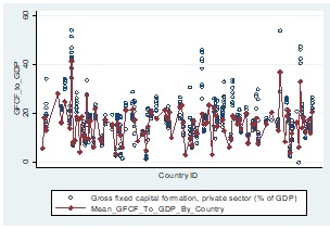
Diagram 2. Mean and Absolute value distribution of GFCF_to_GDP by year 

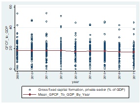
On the other hand, time specific component seems to be insignificant. Namely, as diagram 2 shows, on average, GFCF_to_GDP is not changed over the period significantly. These results support the idea that in our model only country specific effects should be involved while time specific component seems to be not significant.

Our conclusion based on the diagrams 1 and 2 is consistent with the results of Housman test for fixed/random effect models and test for time fixed effect significance (see table 1 and 2 in Appendix). Based on the tests, we use LSDV model with above mentioned independent variables and country specific fixed effects only. The model takes the following form: 

Y_it=α+β₁X_1it+β₂X_2it+β₃X_3it+β₄X_4it+γ_i+u_it 

The key insight while employing this model is that if the unobserved variable does not change over time, then any changes in the dependent variable must be due to influences other than these fixed characteristics (Stock and Watson, 2003, p.289-290). The other factors are independent variables included in the model.

Finally, estimated model with independent variables and country fixed effects has the following form: 

Table 1. Estimation results for LSDV model[3]

References

- Kiviet, J. 1995. On bias, inconsistency, and efficiency of various estimators in dynamic panel data models. Journal of Econometrics 68, 53-78
- Barro R. (1974). “Are government bonds net wealth?” Journal of Political Economy 82(6): 1095-1117.
- Krugman P. 1988. ‘‘Financing vs. Forgiving a Debt Overhang,’’ Journal of Development Economics, Vol. 29 (November), pp. 253–268
- Reinhart M. Rogoff K, (2010) “Growth in a Time of Debt”, American Economic Review: Papers & Proceedings, Vol. 100, No. 2, pp. 573–78
- Schclarek A. (2004), Debt and economic growth in developing and industrial countries, Working Paper no. 34, School of Economics and Management, Lund University.
- Patillo C. Poirson, H. Ricci L. (2004), “What are the channels through which external debt affects growth?” IMF Working Paper no. 15, Washington, D.C
- 10. Blinder A. and Solow R. (1974) Analytical Foundations of Fiscal Policy, pp. 3-115.
- Ricardo D. (1820). "Essay on the Funding System", 1820
- Stock J. H. and Watson M. W., (2003), “Introduction to Econometrics,” New York, Prentice hall; 289-290
- www.WDI.com
- www.IMF.com
- www.WEO.org
[1] The difference between government debt and public debt is that public debt includes liabilities of state owned enterprises which is contingent liabilities for general government.
[2] Financial development index ranges between [0-1] interval. To express as percentage scale, it is multiplied by 100
[3] Diagnostic test for the OLS based estimated model shows that it suffers from heteroscedasticity. So, standard errors calculation for coefficients are based on robust approach.